Vector database Recommender System
Dense vector embeddings make it easy to find similar documents in a dataset. With a document in the embedding space, just look at the other documents that are close, and probably they are related. This is called a k-nearest neighbors (KNN) search. Classic recommender systems such as collaborative filtering require a lot of user data and training. However with pre-trained embedding models you don’t need any training to recommend related documents.
This works well for item-to-item recommendations. But what if you want to recommend something for a specific user. If you want to go to user-to-items recommendations you need some interaction data again. One strategy is to build a user-embedding based on the mean of the embeddings of the documents the user interacted with. A KNN search with this user-embedding will give the results the user is most likely interested in. Erika Cardenas explained this in further detail in her Haystack US 2023 talk. With just a few clicks the user quickly gets nice recommendations without a lot of extra systems if you already have a vector database.
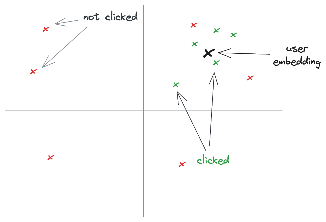
The problem that I’m trying to solve goes a bit deeper. I’ve got a lot of documents that have a certain label (e.g. a brand of a product, some color, language, author of articles). And when the user selects that label we want to show the most interesting documents. But at the moment we only know if that document has the label or not, which doesn’t say anything about how we should rank those documents. Also the documents are refreshed regularly and the number of documents is quite large compared to the number of clicks, so an individual document only gets a few clicks. What we want are the best documents ranked best. Using a similar approach as the user-embedding, we can create a ‘label-embedding’ of clicked documents when users were searching in this category.
One problem of this, contrary to user-embeddings that can be limited to averaging the last few document embeddings the user clicked on, is that we would eventually take the average embedding of many clicked document, and does that actually represent the most popular type of document, or is that some ‘random’ point in the embedding space.
Instead, in the list of all clicked documents, there are probably a few clusters of related documents. The idea is that instead of one average embedding we get a few embeddings, one for each cluster, and for each embedding we do a KNN search, and finally combine the results.
Implementation
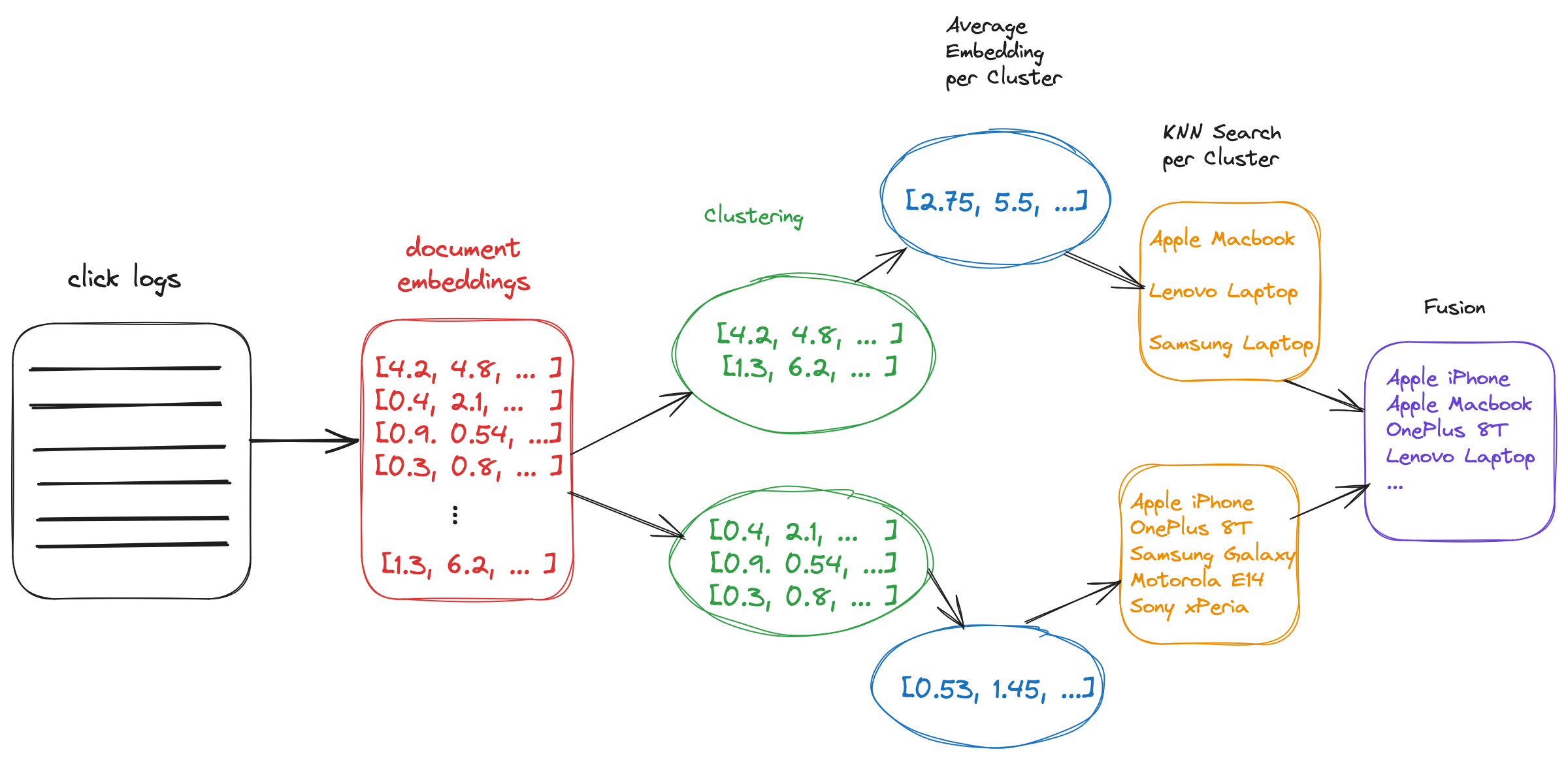
From a high level the pipeline looks as shown in this image. First we collect the relevant click logs, and see which documents are clicked, then we get the embeddings for these documents, and create clusters. For each cluster we do a KNN search to get more related documents (even though that document might not have any interactions yet), combine these lists in a single final list, and finally present that as the ranking to the user.
Clustering
The idea to cluster dense embedding vectors resembles most of what BERTopic does, as described in BERTopic: Neural topic modeling with a class-based TF-IDF procedure by Maarten Grootendorst. From documents it can create embeddings using an embedding model, cluster the embeddings and finally extract the topic description of each cluster. The first and last steps are not necessary for us, we already have the embeddings, and we don’t really need to label the topics, but we can look how it creates clusters from the embeddings.
It uses two steps:
-
Dimension reduction is necessary to prevent the curse of dimensionality. From dense vectors of 384, 768 or sometimes more than 4000 dimensions. That is too much for clustering algorithms to work well. Dimension reduction reduces those higher dimensions to a much lower number, such as 5 or 10 that the clustering algorithm can handle well. If you reduce it further to 2 or 3 dimensions you can also render the vectors in a 2 or 3-dimensional graph. BERTopic uses UMAP over other methods such as PCA or t-SNE because UMAP has shown to preserve more of the local and global features of high-dimensional data in lower projected dimensions.
-
Clustering. For clustering BERTopic uses the HDBSCAN clustering algorithm. Clustering assigns a cluster label to the (reduced) embeddings. Contrary to the KMeans algorithm the number of clusters is dynamic. Compared to the DBSCAN algorithm it works better if the (reduced) embeddings are not homogeneously distributed in the embedding space, so it can also create different clusters in dense areas.
After this process we have cluster labels for all clicked documents, and we can use them to create the ‘cluster-embeddings’ that we will use as center points for our KNN search. I found two methods:
- Find the centroid embedding. This is possible when using a the KMeans clustering algorithm. However the clustering is done on the reduced dimension vectors, so it would need to be mapped back to the original document (embedding).
- Take the mean of all embeddings that fall in this cluster. As HDBSCAN can create non linear clusters (e.g. an inner and an outer circle as two clusters) taking the mean seems a bit weird. But as the means are taken on the original high dimensional vectors it does work OK in practice.
KNN Search
For KNN search we use a vector database. A vector database stores the documents with the document embeddings and provides a way to query the database. A naive way to find the most similar documents of a given vector would be to calculate the similarity for each document with the query vector, and take the k vectors with the highest similarity. This scales linearly and isn’t suited for bigger datasets. Vector databases implement Approximate Nearest Neighbor (ANN) algorithms which makes querying much more efficient (with the cost of being approximate). The most popular algorithm is Hierarchical Navigable Small Worlds (HNSW) and is implemented in vector databases like qdrant, Weaviate or Elasticsearch (that we use).
Note that the vector database needs to support some way of filtering, as the results need to match the initial search constraints (in our case, the document should have a label).
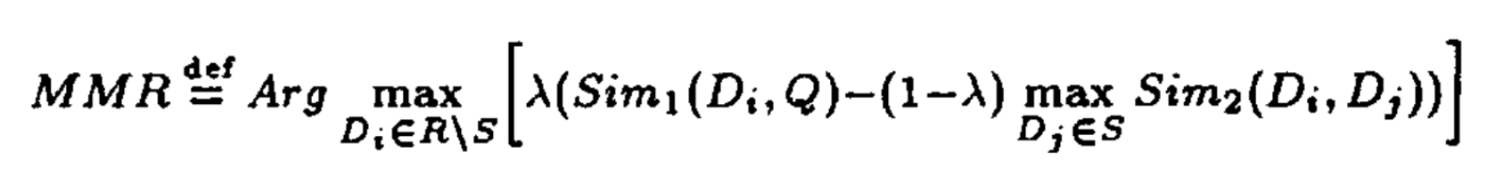
The top-k documents closest to the cluster-embedding are retrieved with the KNN search. These are however the top-k closest to that embedding, but may not be representative for the entire space of the cluster. Especially with e-commerce products there are a lot of variants of the same product, while it might be more relevant to get a diverse set of recommendations for this cluster. The Maximal Marginal Relevance algorithm is an algorithm that can diversify the ranking of the found documents. The algorithm iteratively adds documents to a new list from the original ranked list that best matches the cluster-embedding (or more generally, the query vector), but penalizes documents that are already in the resulting list:
Fusing results from different clusters
After calculating the clusters and cluster embeddings, and retrieving and diversifying potential candidate documents, we have a list of documents for each cluster. However we want to present the user with a final flat list. Reciprocal Rank Fusion (RFF) is a straight forward algorithm that got implemented recently into some vector databases that also implemented hybrid search.
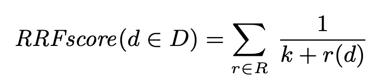
RFF calculates a score based on the rank of the documents in each list. In our case we have lists of documents for each cluster, and the position in that list is the rank for that document. k is a tunable parameter, usually set to 60, that improves the resulting score. As the documents are all in a different cluster each candidate document only is in one of the lists. So initially the score for all first documents will be 1/(60 + 1).
However some clusters are more important than other clusters, some clusters are bigger as more users clicked on documents that are like the documents in that cluster, so we assume those documents should be more relevant. Using the relative sizes of the clusters we can add a weight in the numerator of the fraction.
        num_docs_in_cluster
w = a + -------------------
           total_docs
We can also add a tunable parameter a that makes the cluster size weight more or less important.
                w
Score(d) =  ----------
            k + rank(d)
After computing the score for all documents we can sort them and get the final, diverse, sorted relevant list of documents.
Production concerns
Processing all the click logs and calculating the clusters is a bit compute intensive, and would not work for real time traffic. But we can periodically calculate the cluster embeddings. That’s not a lot of data, basically just one vector for each cluster. Doing the KNN search using a vector database and doing some re-ranking and fusing using MRR and RFF can be done in your web application.
Conclusion
Vector databases with embeddings unlock building a recommender system quickly without a lot of data. Furthermore it can be used for creating rankings in a search engine when there is no natural ranking because the documents either match or not, (a product is in sale or not, an article is written by this author or not, etc.) but there is no way yet in telling if it matches more or less. With click logs we can create an embedding of all the documents that are clicked and get related documents that are most clicked. However, if it’s likely there are more types of documents in the click logs, we create clusters using the UMAP and HDBSCAN dimension reduction and clustering algorithms. Finally with KNN search, optionally some diversification of the results using MRR, and combining the results of each cluster using a modified RFF score, we will get results where documents that were similar to clicked documents will get a higher ranking than documents that are less clicked.